How much of the residual stream is "output token" focused?

That is, how much residual stream space is allocated to output token space? How much is kept for other information.

For this, I am only looking at small models (Qwen2.5-3B and Llama-3.2-3B), and would not want to make predictions on what happens for larger models.

To determine this, I ask the model to complete a prompt, and store the top k token predictions. Each prediction has an associated unembedding vector, and has shape [d_model].

Recall, the unembedding matrix [d_model, vocab_size] is multiplied by the output residual stream, r, at the final layer to produces the logits [vocab_size].

The logits undergo softmax and then sampled. To separate the output subspace, we first construct the output subspace matrix, V, where each column of V is the unembedding vector of our k tokens, and thus has shape [d_model, k].

We now assume we can split the r into two subspaces, the parallel and orthogonal spaces, specifying components parallel to this output subspace, and orthogonal.

r = r_parallel + r_orthogonal.

This way, r_orthogonal does not affect output predictions for these k tokens in any meaningful way - we could make r_orthogonal 10x stronger, and we would get the same relative predictions among our top k tokens. Note that r_orthogonal can still project onto other tokens in the vocabulary outside our chosen k.

Our matrix of unembedding vectors need not be orthogonal or normalised (orthonormal), and so we use a QR decomposition:

Q, R = torch.linalg.qr(V)

where Q is [d_model, k] and R is [k, k]

Q is now our orthonormal version of V, it spans the same subspace (we can construct any vector with either Q or V) but Q is normalised and orthogonal.

To project our residual stream r onto the output subspace spanned by V (and Q) we compute r_parallel = Q @ (Q^T @ r)

Where (Q^T @ r) determines the projection of r along the columns of Q (our normalised output unembedding vectors, shape [k]) and therefore multiplying by Q gives the correct shape [d_model]. This step takes our residual stream vector, and decomposes the output unembedding vector and rewrites it into this new basis defined by Q.

So, r_parallel will have nonzero elements that describe how much the stream has components along unembedding vectors. The remaining residual stream subspace:

r_orthogonal = r - r_parallel defines a subspace that is orthogonal to the output unembedding vector subspace.

The norm of these subspaces can be thought of as a heuristic for how much r allocates to the top k token predictions versus other tokens in the vocabulary.

By finding the ratio norm(r_parallel)/norm(r_orthogonal) we can get an idea of the fraction of r that is focused on predicting these top k tokens.

Is this decomposition actually meaningful?

Before looking at results, an important sanity check: is the projection onto the output subspace actually special, or would we see similar numbers for any random k-dimensional subspace? To test this, I compared the output subspace (top 30 tokens) against a random 30-dimensional subspace made from orthonormalized random vectors.

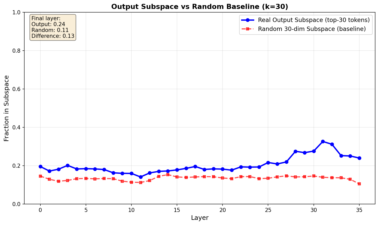
The output subspace projects at roughly 24% by the final layer, while the random baseline sits around 11%. So the output subspace shows about 2x the projection compared to random - this suggests the decomposition is picking up on real structure. Interestingly, the fact that it's only 24% (not 50%+) implies the residual stream genuinely is doing other work beyond just preparing the output token.

Initial Results

I tried a few prompts, and the general theme holds. For k = 30, the ratio of output focused to orthogonal is around 20% in the early layers. At about 75% of the way through the forward pass, the ratio increases slightly and maximises at about 40%

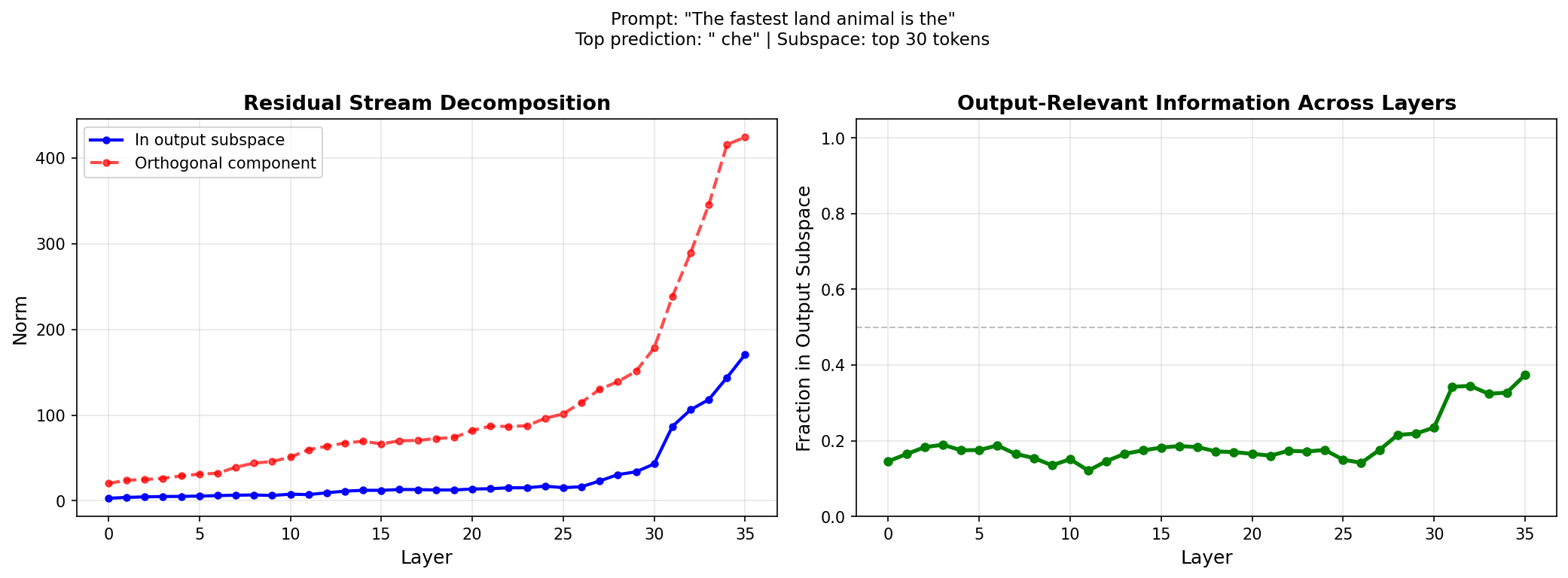
To me, this suggests at layer 1 the model already has a slight understanding of its output prediction subspace, and only about 75% of the way through, does it start to refine these predictions, but this effect is still subtle, there is not apparent "jump" in output focused predictions.

Again, this might be due to the model already having an idea from layer 1, which it refines. As these examples are all rather simple prediction examples, this could be likely.

Does complexity matter?

Since the initial prompts were simple factual completions, I tested whether more complex prompts requiring reasoning would show different patterns.

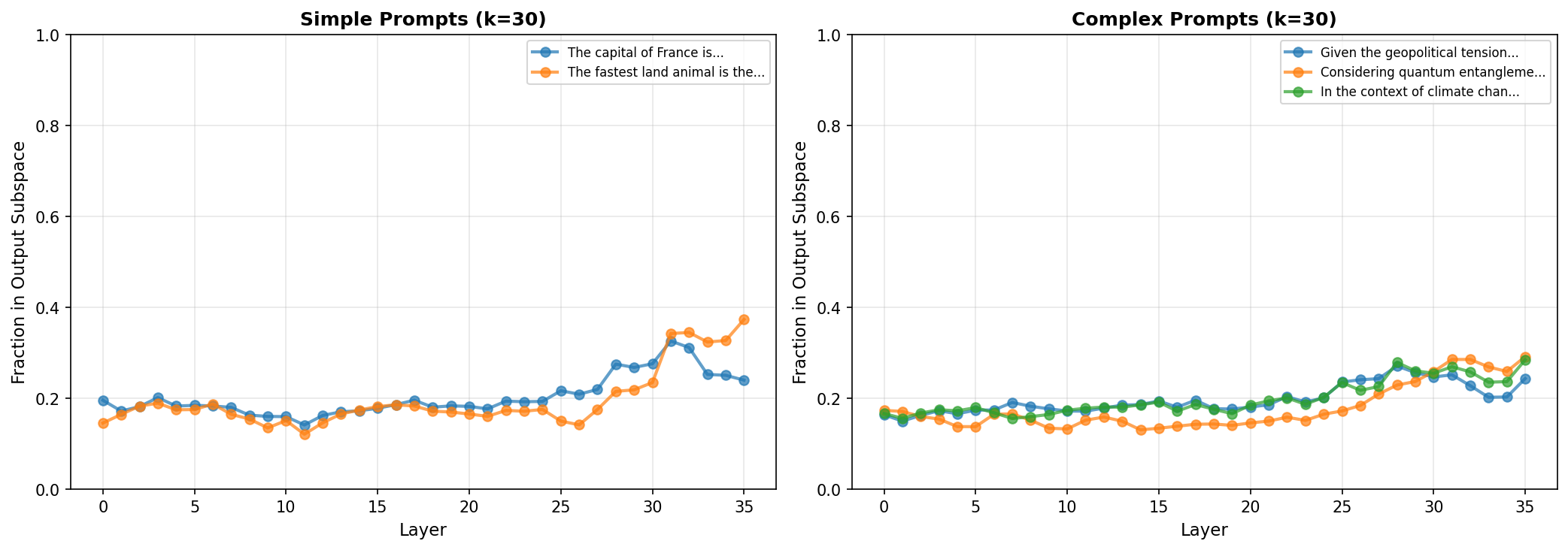
Turns out, not really. Both simple and complex prompts hover around 15-20% in early layers and rise to 25-35% by the end. This was surprising - maybe complex reasoning happens primarily in the orthogonal subspace (the 70-80% that doesn't point at output tokens), and only the final "answer selection" happens in output space. The model might be doing reasoning in some abstract feature space, then converting to tokens late in the network.

Finding the right k: saturation analysis

If you run this analysis with k = 1000, the ratio starts at around 70%, and stays roughly constant with a slight reduction until the final layer where it kicks up

This shows what happens with oversaturation (when k is much larger than the number of plausible output tokens). For these simple prompts, there are maybe 5-10 genuinely likely output tokens, so k=1000 includes hundreds of irrelevant token directions. The ratio starts at ~70% (much higher than k=30's ~20%) because we're now capturing weak projections onto many unlikely tokens. The characteristic late-layer increase still happens, but it's compressed into a narrower range, making the pattern less informative. This is why choosing k too large washes out the signal.

To find where saturation kicks in, I systematically tested k values from 10 to 200:

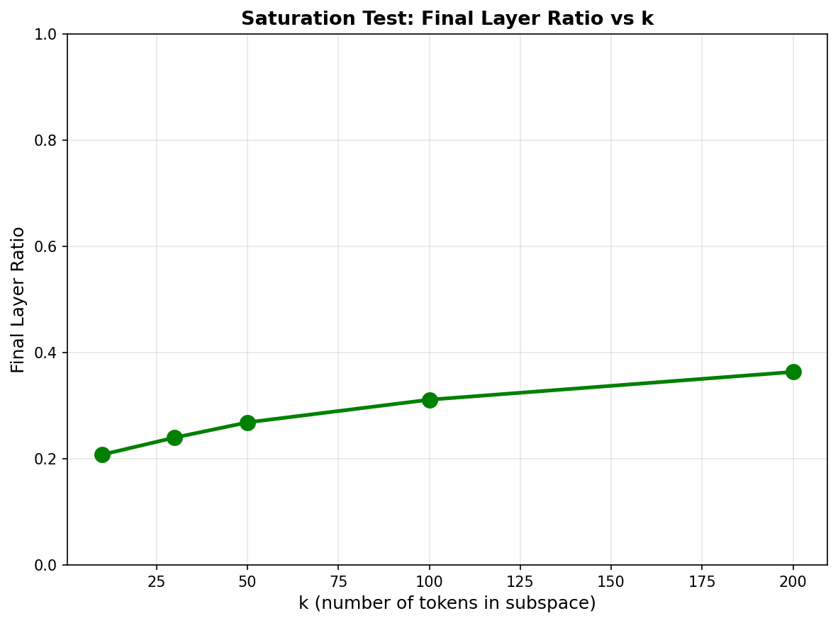
The curve is smooth rather than sharp. At k=30 we get ~24%, at k=200 only ~37%. This backs up the claim that k=1000 oversaturates. The k=30 choice seems reasonable: big enough to capture the real output subspace, small enough to avoid including irrelevant tokens.

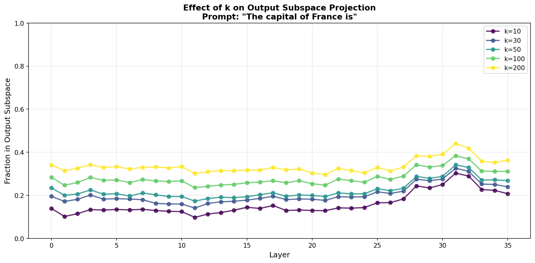
Looking at how different k values evolve through layers, the pattern holds across all k: flat in early/middle layers, uptick around layer 27-30. Higher k just shifts everything up somewhat proportionally.

Homonyms: same token, different meanings

What if the next predicted token is the same, and the token predicted is a word that has different meanings? E.g. a Homonym.

For the following examples, I show the residual stream similarity (measured using cosine similarity) of prompts that predict the same token but with different semantic contexts. Cosine similarity ranges from -1 to 1, where 1 means identical direction, 0 means orthogonal, and -1 means opposite.

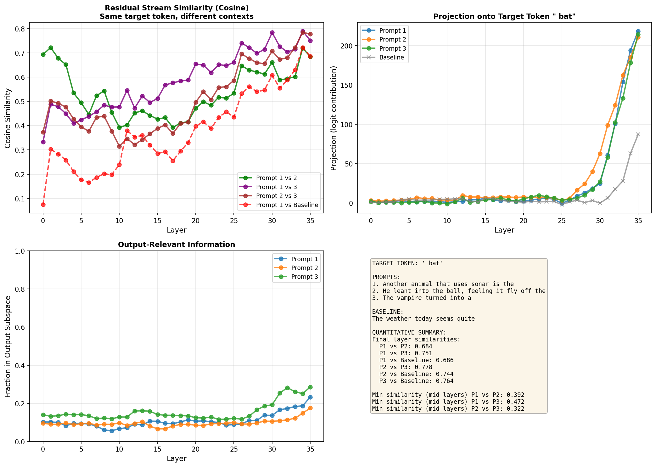
Bat

prompts = ["Another animal that uses sonar is the", "He leant into the ball, feeling it fly off the", "The vampire turned into a"]

baseline_prompt = "The weather today seems quite"

target_token = " bat"

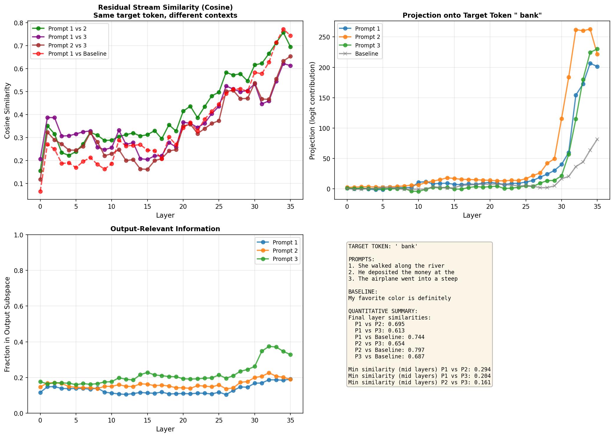
Bank

prompts = ["She walked along the river", "He deposited the money at the", "The airplane went into a steep"]

baseline_prompt = "My favorite color is definitely"

target_token = " bank"

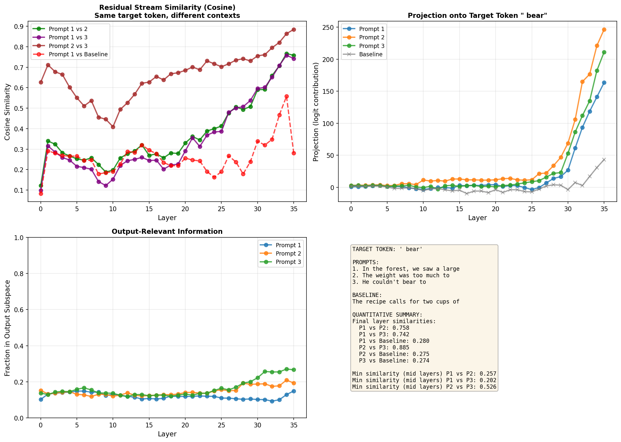
Bear

prompts = ["In the forest, we saw a large", "The weight was too much to", "He couldn't bear to"]

baseline_prompt = "The recipe calls for two cups of"

target_token = " bear"

What the homonym results show

All three homonyms show a somewhat U-shaped pattern. Initially the prompts with the same target token are more similar to each other (0.3-0.7 cosine similarity) than to the baseline. This makes sense, that 20% of the residual stream that's output-focused is already pointing towards " bat" (or " bank", or " bear"), giving a higher dot product compared to baseline where those 20% point elsewhere.

As the layers progress, the pairwise similarities drop - sometimes quite dramatically. For "bank", the minimum mid-layer similarity between prompts gets as low as 0.16, compared to initial values around 0.3-0.4. This might be the model exploring and maximising the semantic differences.

Towards the final layers, similarities rise again. By layer 36, prompts predicting the same token converge back to 0.6-0.9 similarity. The baseline comparisons also increase at the end, too. This supports the idea that streams generally become more aligned in final layers (likely from pre-training optimization), but the shared output target creates additional convergence for the homonym pairs.

The quantified mid-layer minimums (listed in the bottom-right of each plot) give concrete evidence of semantic divergence: 0.32-0.47 for bat, 0.16-0.29 for bank, 0.20-0.26 for bear. These aren't tiny effects, the model is doing something different in the middle layers despite heading toward the same output. This is an expected result, but is nice to see in practise.

Summary

For these small models, roughly 20-25% of the residual stream appears focused on the top 30 output tokens in early layers, rising to 25-40% by the final layers. This was validated against a random baseline, which only showed ~11% projection.

The uptick happens around layer 27-30 (about 75% through the network), and this pattern holds whether the prompt is simple or complex. Complex reasoning probably happens in the orthogonal 70-80% of the residual stream, with only the final answer selection happening in output space.

Homonym analysis reveals clear semantic processing: prompts predicting the same token start with moderate similarity, diverge in middle layers as meanings are disambiguated, then converge again in final layers as the model commits to the shared output (but so too does the baseline similarity).

The k=30 choice appears optimal for this analysis - k=10 is too restrictive, k=200+ starts oversaturating, and k=1000 completely washes out the signal.

Future Work

This work is by no means exhaustive, there is likely substantial statistical uncertainty, and there are likely other effects going on. I will try and chip away at some questions I have in time.

AI assisstance

This work was heavily influenced by AI. In particular, Opus 4.5 wrote ~50% of the code for this project, and ~100% of the plotting code.

I also used Opus 4.5 to discuss some of the key findings in this work, in order to cement my understanding.